import altair as alt
import pandas as pd
import ppscore as pps
from pycaret.classification import *
import shap
from sklearn.metrics import average_precision_score
from sklearn.model_selection import train_test_split
from ydata_profiling import ProfileReport


# customize Altair
def y_axis():
    return {
        "config": {
            "axisX": {"grid": False},
            "axisY": {
                "domain": False,
                "gridDash": [2, 4],
                "tickSize": 0,
                "titleAlign": "right",
                "titleAngle": 0,
                "titleX": -5,
                "titleY": -10,
            },
            "view": {
                "stroke": "transparent",
                # To keep the same height and width as the default theme:
                "continuousHeight": 300,
                "continuousWidth": 400,
            },
        }
    }


alt.themes.register("y_axis", y_axis)
alt.themes.enable("y_axis");Predicting diabetes with Pima Indians

Objectives
- Example end-to-end supervised learning workflow with Pima Indians
- Focus on conceptual understanding of machine learning
- Demonstrate use of Predictive Power Score (PPS)
- Demonstrate capabilities of low-code tools
- Demonstrate use of
average_precision_score(link) - Demonstrate SHAP values
Attribution
Dataset
- Pima Indians paper (original paper)
- Kaggle datacard (link)
Python libraries
- Altair (docs)
- ydata-profiling (docs)
- Predictive Power Score (PPS, GitHub, blog)
- PyCaret: open-source, low-code machine learning library in Python that automates machine learning workflows (link)
Read and explore the data
%%time
df = pd.read_csv("diabetes.csv").astype({"Outcome": bool})
train, test = train_test_split(df, test_size=0.3)
profile = ProfileReport(train, minimal=True, title="Pima Indians Profiling Report")
profile.to_file("pima-indians-profiling-report-minimal.html")
CPU times: user 5.54 s, sys: 184 ms, total: 5.72 s
Wall time: 1.7 sprofile.to_notebook_iframe()Investigate features with largest predictive power
We use the Predictive Power Score to evaluate which features have the highest predictive power with respect to Outcome.
predictors = (
    pps.predictors(train, "Outcome")
    .round(3)
    .iloc[:, :-1]
)
base = (
    alt.Chart(predictors)
    .encode(
        y=alt.Y("x:N").sort("-x"),
        x="ppscore",
        tooltip=["x", "ppscore"],
    )
)
base.mark_bar() + base.mark_text(align="center", dy=-5)
Investigate colinearity
pps.matrix(train)| x | y | ppscore | case | is_valid_score | metric | baseline_score | model_score | model | |
|---|---|---|---|---|---|---|---|---|---|
| 0 | Pregnancies | Pregnancies | 1.000000 | predict_itself | True | None | 0.000000 | 1.000000 | None |
| 1 | Pregnancies | Glucose | 0.000000 | regression | True | mean absolute error | 23.651769 | 24.024994 | DecisionTreeRegressor() |
| 2 | Pregnancies | BloodPressure | 0.000000 | regression | True | mean absolute error | 12.748603 | 12.961633 | DecisionTreeRegressor() |
| 3 | Pregnancies | SkinThickness | 0.000000 | regression | True | mean absolute error | 13.467412 | 13.630828 | DecisionTreeRegressor() |
| 4 | Pregnancies | Insulin | 0.000000 | regression | True | mean absolute error | 79.240223 | 85.015086 | DecisionTreeRegressor() |
| ... | ... | ... | ... | ... | ... | ... | ... | ... | ... |
| 76 | Outcome | Insulin | 0.000000 | regression | True | mean absolute error | 79.240223 | 84.802415 | DecisionTreeRegressor() |
| 77 | Outcome | BMI | 0.035133 | regression | True | mean absolute error | 5.672812 | 5.473511 | DecisionTreeRegressor() |
| 78 | Outcome | DiabetesPedigreeFunction | 0.000000 | regression | True | mean absolute error | 0.226384 | 0.234531 | DecisionTreeRegressor() |
| 79 | Outcome | Age | 0.000000 | regression | True | mean absolute error | 8.888268 | 8.997094 | DecisionTreeRegressor() |
| 80 | Outcome | Outcome | 1.000000 | predict_itself | True | None | 0.000000 | 1.000000 | None |
81 rows × 9 columns
pps_matrix = (
    pps.matrix(
        train.loc[:, predictors.query("ppscore > 0")["x"].tolist()],
    )
    .loc[:, ["x", "y", "ppscore"]]
    .round(3)
)
(
    alt.Chart(pps_matrix)
    .mark_rect()
    .encode(
        x="x:O",
        y="y:O",
        color="ppscore:Q",
        tooltip=["x", "y", "ppscore"])
).properties(width=500, height=500)
Build models
cls = setup(data = train,
             target = 'Outcome',
             numeric_imputation = 'mean',
             feature_selection = False,
             pca=False,
             remove_multicollinearity=True,
             remove_outliers = False,
             normalize = True,
             )
add_metric('apc', 'APC', average_precision_score, target = 'pred_proba');| Description | Value | |
|---|---|---|
| 0 | Session id | 5752 |
| 1 | Target | Outcome |
| 2 | Target type | Binary |
| 3 | Original data shape | (537, 9) |
| 4 | Transformed data shape | (537, 9) |
| 5 | Transformed train set shape | (375, 9) |
| 6 | Transformed test set shape | (162, 9) |
| 7 | Numeric features | 8 |
| 8 | Preprocess | True |
| 9 | Imputation type | simple |
| 10 | Numeric imputation | mean |
| 11 | Categorical imputation | mode |
| 12 | Remove multicollinearity | True |
| 13 | Multicollinearity threshold | 0.900000 |
| 14 | Normalize | True |
| 15 | Normalize method | zscore |
| 16 | Fold Generator | StratifiedKFold |
| 17 | Fold Number | 10 |
| 18 | CPU Jobs | -1 |
| 19 | Use GPU | False |
| 20 | Log Experiment | False |
| 21 | Experiment Name | clf-default-name |
| 22 | USI | 10e4 |
%%time
best_model = compare_models(include=["et", "lightgbm", "rf", "dt"], sort="APC")| Model | Accuracy | AUC | Recall | Prec. | F1 | Kappa | MCC | APC | TT (Sec) | |
|---|---|---|---|---|---|---|---|---|---|---|
| et | Extra Trees Classifier | 0.7569 | 0.8039 | 0.5090 | 0.6832 | 0.5719 | 0.4106 | 0.4261 | 0.6795 | 0.1740 |
| rf | Random Forest Classifier | 0.7412 | 0.7893 | 0.5013 | 0.6420 | 0.5538 | 0.3784 | 0.3896 | 0.6661 | 0.0330 |
| lightgbm | Light Gradient Boosting Machine | 0.7252 | 0.7776 | 0.5090 | 0.5987 | 0.5452 | 0.3519 | 0.3574 | 0.6378 | 0.1310 |
| dt | Decision Tree Classifier | 0.6691 | 0.6275 | 0.5019 | 0.5002 | 0.4904 | 0.2503 | 0.2559 | 0.4269 | 0.0050 |
CPU times: user 537 ms, sys: 135 ms, total: 672 ms
Wall time: 3.96 s
Evaluation
predictions = (
    predict_model(best_model, data=test.iloc[:, :-1])
)
predictions.head()| Pregnancies | Glucose | BloodPressure | SkinThickness | Insulin | BMI | DiabetesPedigreeFunction | Age | prediction_label | prediction_score | |
|---|---|---|---|---|---|---|---|---|---|---|
| 752 | 3 | 108 | 62 | 24 | 0 | 26.000000 | 0.223 | 25 | 0 | 0.76 |
| 295 | 6 | 151 | 62 | 31 | 120 | 35.500000 | 0.692 | 28 | 0 | 0.57 |
| 532 | 1 | 86 | 66 | 52 | 65 | 41.299999 | 0.917 | 29 | 0 | 0.88 |
| 426 | 0 | 94 | 0 | 0 | 0 | 0.000000 | 0.256 | 25 | 0 | 0.89 |
| 68 | 1 | 95 | 66 | 13 | 38 | 19.600000 | 0.334 | 25 | 0 | 0.97 |
evaluate_model(best_model)SHAP
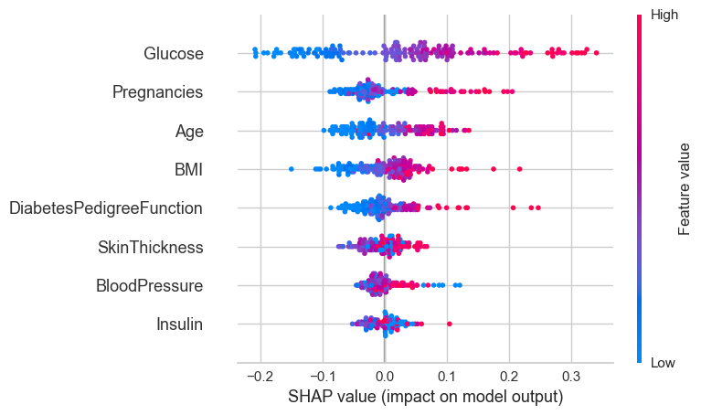
interpret_model(best_model)
interpret_model(best_model, plot="reason", observation=1)
Visualization omitted, Javascript library not loaded!
Have you run `initjs()` in this notebook? If this notebook was from another user you must also trust this notebook (File -> Trust notebook). If you are viewing this notebook on github the Javascript has been stripped for security. If you are using JupyterLab this error is because a JupyterLab extension has not yet been written.
Have you run `initjs()` in this notebook? If this notebook was from another user you must also trust this notebook (File -> Trust notebook). If you are viewing this notebook on github the Javascript has been stripped for security. If you are using JupyterLab this error is because a JupyterLab extension has not yet been written.
interpret_model(best_model, plot="reason")
Visualization omitted, Javascript library not loaded!
Have you run `initjs()` in this notebook? If this notebook was from another user you must also trust this notebook (File -> Trust notebook). If you are viewing this notebook on github the Javascript has been stripped for security. If you are using JupyterLab this error is because a JupyterLab extension has not yet been written.
Have you run `initjs()` in this notebook? If this notebook was from another user you must also trust this notebook (File -> Trust notebook). If you are viewing this notebook on github the Javascript has been stripped for security. If you are using JupyterLab this error is because a JupyterLab extension has not yet been written.
